Mamba - Linear-Time Sequence Modeling with Selective State Spaces

Introduction

Foundation models are large models pre-trained on massive data and then adapted for downstream tasks. FMs often employ sequence models as the backbone and are currently predominantly based on the Transformer.

The efficacy of self-attention in the Transformer attributed to

• the ability to route information densely within a context window

However, this property also brings in fundamental drawbacks

• the inability to model anything outside of the finite context window
• quadratic scaling with respect to the window length

Recently, structured state space sequence models (SSMs) were proposed as a new class of architectures for sequence modeling. These models can be interpreted as a combination of RNNs and CNNs, with inspiration from classical state space models.

The obtained results from SSMs are very promising, as it not only scale linearly or near-linearly with respect to the sequence length but also demonstrates outstanding ability in modelling long-range dependencies, dominating benchmarks such as the Long Range area.

In addition, many variations of SSMs have been successful in continuous signal data domains such as audio and vision. However, SSMs have been less effective in modeling discrete and information dense data such as text.

Therefore, the authors propose a new class of SSM to achieve the performance of Transformers while scaling linearly.

Selection Mechanism

Previous SSMs lacks the ability to select data in an input-dependent manner. A new selection mechanism is proposed to to allow the model to filter out irrelevant information and remember releveant information indefinitely.

Hardware-aware Algorithm

To overcome the requirement where all prior models must be time- and input-invariant to be computationally efficient, the authors propose a hardware-aware algorithm. Instead of computing the model convolutionally, the algorithm computes the model recurrently with a scan and does not materialize the expanded state to avoid IO access between different GPU Mem hierarchy.

Architecture

The authors simplify the prior SSM architectures by combining the prior SSM architectures with the MLP block of Transformers into a single block (Mamba).

Selective SSMs and by extension the Mamba architecture are fully recurrent models with key properties such as

1. High Quality for dense modalities such as language and genomics
2. Fast Training and Inference as training computation and memory scales linearly and inference autoregressive unrolling requires constant time per step.
3. Long Context as model demonstrated quality and efficiency for sequence length up to 1M

State Space Models

Structured state space models (S4) is a recent class of sequence models for deep learning that are related to RNN, CNN, and classical state space models. They are defined with four parameters $(\Delta, A, B, C)$and are inspired by a continuous system

$\begin{aligned} h^\prime(t) &= Ah(t) + B(x(t)) && \text{(1a)} \\ y(t) &= Ch(t) && \text{(1b)} \end{aligned}$

that maps a 1-dimensional function or sequence $x(t)\in \R \mapsto y(t) \in \R$ through an implicit latent space $h(t) \in \R^N$.

Currently, the S4 models use the four parameters to define a sequence-to-sequence transformation in two stages:

1. Discretization - the first stage that transforms the “continuous parameters” $(\Delta,A,B)$ to “discrete parameters” $(\bar{A}, \bar{B})$ through fixed formulas $\bar{A} = f_A(\Delta,A)$ and $\bar{B} = f_B(\Delta,A,B)$, where $(f_A,f_B)$ is a discretization rule. Various rules can be used. Below is an exmpler rule using the zero-order hold (ZOH):

$\bar{A} = \exp(\Delta A) \quad \bar{B} = (\Delta A)^{-1}(\exp(\Delta A) - I) \cdot \Delta B$

1. Computation - after the parameters are discretized, the model can be computed two ways, either as a linear recurrence (2) or a global convolution (3). The model uses the convolutional mode (3) for efficient parallelizable training and recurrent mode (2) for efficient autoregressive inference.

$\begin{aligned} h_t &= \bar{A}h_{t-1} + \bar{B}x_t & (2a) && && && &\bar{K} = (C\bar{B}, C\bar{AB}, \dots, C\bar{A}^k\bar{B}, \dots) & (3a) \\ y_t &= Ch_t & (2b) && && && &y = x * \bar{K} & (3b) \end{aligned}$

Limitations to State Space Models

Linear Time Invariance

A key property of equations (1), (2), and (3) is Linear Time Invariance (LTI). This means that $(\Delta, A, B, C)$ and $(\bar{A}, \bar{B})$ are fixed for all time-steps. However, LTI models have fundamental limitations in modeling in certain types of data. Thus, the authors propose a method that removes the LTI constraints while overcoming the efficiency bottlenecks.

Efficiency Bottleneck

In addition, the structured SSMs are so named because it requires imposing structure on $A$ matrix to compute efficiently. Commonly, $A$ is imposed to be a diagonal matrix. In this case, $A\in \R^{N\times N}, B \in \R^{N\times1}, C \in \R^{1\times N}$ can all be represented by $N$ numbers.

Consider an input sequence $x$ of batch size $B$ and length $L$ with $D$ channels, the SSM is independently applied to each channel. Then, the total hidden spaces have $DN$ per input, and computing over the sequence length requires $O(BLDN)$ time and memory. This is the root of the efficeincty bottleneck.

Selective State Space Models

This section is dedicated to explain the selection mechanism, its motivation and implementation.

Motivation: Selection as a Means of Compression

The fundamental problem of sequence modeling is compressing context into a smaller state. This problem can be viewed as the tradeoffs between effectiveness and efficiency. For example, attention is effective and inefficient because it explicitly does not compress context at all. On the other hand, recurrent models are efficient due to finite number of states, limiting its effectiveness by how well the state has compressed the context.

To understand the tradeoff, we focus on two examples of synthetic tasks

• Selective Copying: a modification on the popular Copying task by varying the position of the tokens to memorize. This task requires content-aware reasoning to be able to memorize the relevant tokens and filter out irreleant ones.
• Induction Heads: a well-known mechanism hypothesized to explain the majority of in-context learning abilities of LLMs. This tasks also requires content-aware reasoning to know when to produce the correct output in the appropriate context.

The above tasks reveal the failures of LIT models

• Recurrent view: the constant dynamics, for example the transitions $(\bar{A}, \bar{B})$ is not capable of selecting the correct information from the context and cannot pass the hidden state in an input-dependent way.
• Convolutional view: unlike the vanilla Coping task which can be solve by global convolution as it only requires time-awareness, LTI models fail the Selective Copying task due to the lack of content-awareness.

In summary, the efficiency vs. effectiveness tradeoff can be characterized by how well the model compress the states.

• Efficient models must have a small state
• Effective models must have a state that contains all necessary information from the context

To tackle this tradeoff, the authors propose a fundamental principle called selectivity, which is the ability to focues relevant information and filter out irrelevant information.

Improving SSMs with Selection

The authors incorporate a selection mechanism into models by allowing the parameters to affect interactions to be input-dependent. Therefore, the main difference is simply making parameters $\Delta, B, C$ be functions of input.

In particular, the parameters are not of length $L$, meaning that the model has now change from time-invariant to time-varying.

Efficient Implementation of selective SSMs

The core limitation to prior SSMs is their computational efficient, which is also the reason why previous models used LTI (non-selective) models.

Motivation of Prior Models

• Balance a tradeoff between expressivity and speed: we want to maximize hidden state dimension without paying speed and memory cost
• Note recurrent mode is more flexible than the convolutional mode. However, this would require computing and materializing the latent state $h$ with shape $(B, L, D, N)$, much larger than the convolution kernel of $(B, L, D)$.
• Prior LTI SSMs leverage the dual recurrent-convolutional forms to increase the effective state dimension by a factor of $N$ without paying efficieny penalties compared to traditional RNNs.

Overview of Selective Scan: Hardware-Aware State Expansion

The authors address the computation problem of SSMs with three classical techniques: kernel fusion, parallel scan, and recomputation. First, the authors make two main observations:

1. Recurrent computation uses $O(BLDN)$ FLOPS while convolutional computation uses $O(BLD\log(L))$ FLOPs. Therefore, for long sequences and not-too-large state dimension $N$, recurrent actually uses fewer FLOPs.
2. The two challenges are sequential nature of recurrence and the large memory usage. To address the later, we can not materialize the full state $h$.

The main idea is to only materialize the state $h$ only in more efficient levels of memory hierarchy by levearing properties of modern accelerators. In particular, most operations are bounded by memory bandwidth, including our scan operation. We use kernel fusion to reduce the amount of memory IOs, significantly speeding up the process implementation.

More specifically,

• To prepare the scan input $(\bar{A}, \bar{B})$ of size $(B, L, D, B)$, we load SSM parameters $(\Delta, A, B, C)$ from slow High Bandwith Memory (HBM) to fast SRAM, perform discretization and recurrence, and then move back output of size $(B,L,D)$ back to HBM.
• The process is parallelized with a work-efficient parallel scan algorithm to avoid sequential recurrence.
• Employ recomputation to reduce the memory requirements by avoiding saving the intermediate states.

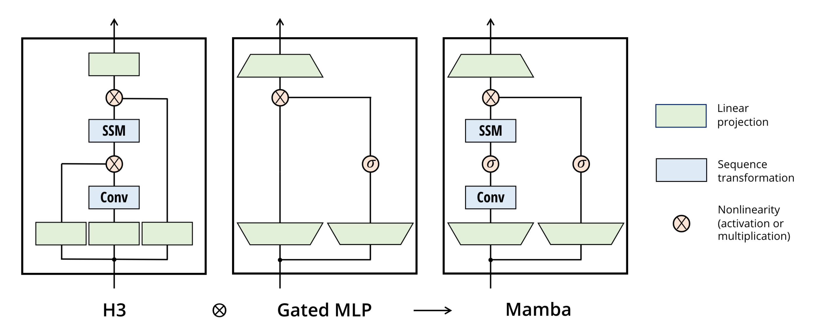
A Simplified SSM Architecture

Similar to other SSMs, selective SSMs are standalone sequence transformations that can be flexibly incorporated into neural networks. Previously, the most well-known SSM architecture is the H3 architecture, which is comprised of a block inspired by linear attention interleaved with an MLP block. This work simplifies the above architecture by combining those two components into one.

The architecture expands the model dimension $D$ by a controllable expansion factor $E$. Most of the parameters ($3ED^2$) are in the linear projections, while the number of SSM parameters is much less in comparison.

The Mamba blcok is repeated, interleaved with standard normalization and residual connections, to form the Mamba architecture. In the experiment, the authors fix $E=2$ with two stacks of the block. SiLu / Switch activation function and LayerNorm are chosen for the activation function and optional normalization layer respectively.

Properties of Selection Mechanisms

Connection to Gating Mechanism

An article helpful for understand gating can be found here.

Note that the connection between RRN gating and the discretization of continuous-time systems is well established. Theorem 1 essentially states that an input-dependent gate can be viewed as the ZOH discretization.

Theorem 1. When $N=1, A=-1, B=1, s_\Delta = \text{Linear}(x), \tau_\Delta = \text{softplus}$, then the selective SSM recurrence takes the form

$\begin{aligned} g_t &= \sigma(Linear(x_t)) \\ h_t &= (1-g_t)h_{t-1}+g_tx_t \end{aligned}$

Interpretation of Selection Mechanisms

Variable Spacing Selectivity allows filtering out irrelevant noise tokens that may occur between inputs of interests, which is exemplified by the Selective Copying task.

Filtering Context Many sequence models do not improve with longer context due to their inability to effectively ignore irrelevant context. On the other hand, selective models can simply reset their state at any time to remove extraneous history, improving the performance with longer context length.

Boundary Resetting In case of multiple independent sequences are stitched together, Transformers can keep them separate by instantiating a particular attention mask. LTI models, on the other hand, will bleed information between sequences. Selective SSMs resets their state at boundaries.

Interpretation of $\Delta$ $\Delta$ in general controls the balance between how much to focus or ignore the current input.

• A large $\Delta$ results the state $h$ and focuses on current input $x$.
• A small $\Delta$ persists the state and ignores the current input.

Interpretation of $A$ The selectivity in $\Delta$ is enough to ensure the selectivity in $(\bar{A}, \bar{B})$. Making $A$ is hypothesized to have similar performance, thus left out for simplicity.

Interpretation of $B$ and $C$ Modifying $B$ and $C$ allows fine-grained control over whether to let an input $x_t$ into the state $h_t$ or the state $h_t$ into the output $y_t$. These can be interpreted as allowing the model to modulate the recurrent dynamics based on the content (input) and context (hidden states) respectively.

Additional Information

Previously, most SSMs use complex numbers in state $h$. However, it has been empirically observed that completely real-valued SSMs seem to work fine, possibly better in some settings. The author hypothesizes that the complex-real tradeoff is related to the continuous-discrete spectrum in data modalities, where

• Complex numbers are helpful for continuous modalities (audio, video)
• Complex numbers are not helpful for discrete modalities (text, DNA)